Chapter 4: Bayesian inference
The steps of Bayesian inference
To make inferences (‘conclusions reached on the basis of evidence and reasoning’) about a hypothesis or unknown parameters, Bayesian inference can be used. Bayesian inference is the method of statistical inference, that uses Bayes theorem, to update the probability estimate about the hypothesis or unknown parameters. This process follows three steps:
Step 1: Choose a prior
This first step of Bayesian inference requires choosing a so called prior (or prior probability distribution/density). The prior represents the initial belief about the hypothesis or the possible values of the parameters before observing the data y. Imagine if we want to predict the weather for tomorrow, our prior can consist of the weather’s data from the last few days. During this chapter, we will give the priors needed for examples. In Chapter 5 more information about priors; how to choose them and how to use them in an analytical manner will be explained.
This prior is defined as p ( \(\theta\) | x). Here \(\theta\) is the unknown parameter we want to make inferences about and x is data given a different hypothesis and parameter values.
Step 2: Choose a statistical model
We need to choose a generative model about the observed data given the data x. This model is then defined by y \(\sim\) p ( \(\theta\) , x). By doing this, we determine the likelihood: \(\mathcal{L}\) (y | \(\theta\) , x). In our example of determining the weather for tomorrow, we can see the likelihood like this: If it’s cloudy today, the likelihood would quantify how much this piece of evidence supports or contradicts our prior belief about the weather.
Step 3: Calculate the posterior density
The final step of Bayesian inference consists of updating the prior of step 1 by using the found likelihood in step 2. By combining the prior and likelihood, we obtain the posterior density. The posterior density is defined as: Posterior \(\propto\) Prior x Likelihood. Or written in the prior (p ( \(\theta\) | x)) and likelihood (\(\mathcal{L}\) (y | \(\theta\) , x )) we determined in respectively steps 1 & 2:
\begin{equation} p ( \theta | y , x) \propto p ( \theta | x) \cdot \mathcal{L} (y | \theta , x) \tag{4.1} \end{equation}
We can calculate the posterior p ( \(\theta\) | y , x) by applying Bayes theorem, which we defined in Chapter 3 as P(A | B) = \(\frac{P ( B | A ) P ( A )}{P ( B )}\).
Visual example
Imagine a doctor wants to diagnose a patient for a rare disease. A research found that 1 out of 1000 people have this disease (so 0.1% of the population). The doctor created a test to find out if his patient has the disease. It is determined that the test is 99% accurate if the patient has the disease and gives out a false positive 5% of the times. After testing the patient, the test gives a positive result (this is the data y that we can observe). Now it is up to us to determine the probability of the patient actually having the disease.
By using Bayesian inference, we can update our prior estimate that the probability of the patient having the disease is 0.1%. We do this by using the given data x about the test to create a likelihood. With this prior and the found likelihood, we can then determine the posterior and posterior probability using Bayes Theorem. See how this is done in the code below. Try to see if you understand the steps we take!
[13]:
# -------------------- Visual example --------------------
import numpy as np

# Step 1: Prior
Prior_Disease = 0.001 # The probability for the patient having the disease is 0.1%. (P(Disease) = 0.001)
Prior_NoDisease = 1-Prior_Disease # The probability for the patient not having the disease is 99.9%. (P(No Disease) = 0.999)

# Step 2: Model and likelihood
Positive_Disease = 0.99 # The probability that if you test positive, you have the disease is 99%. (P(Positive|Disease) = 0.99)
Positive_NoDisease = 0.05 # The probability that if you test positive, you don't have the disease (false positive) is 5%. (P(Positive|No Disease) = 0.05)
Positive = (Positive_Disease * Prior_Disease) + (Positive_NoDisease * Prior_NoDisease) # The probability of having a positive test.

# Step 3: Posterior probability
# Computing this by using Bayes' theorem : P(Disease|Positive) = (P(Positive|Disease)*P(Disease)) / P(Positive)
Disease_Positive = (Positive_Disease*Prior_Disease)/Positive # The probability that you have the disease if you test positive.

# This gives us the following result:
print("The posterior probability of the patient having the disease if they test positive is", (np.round(Disease_Positive,4))*100,
      "%, while initially the chances of the patient having the disease was", (np.round(Prior_Disease,3))*100,"%.")
The posterior probability of the patient having the disease if they test positive is 1.94 %, while initially the chances of the patient having the disease was 0.1 %.
This is ofcourse a very small probability. If this feels weird, just remember that the chances of having the disease are small and that the false positivity of the test impacts the probability significantly as well. Also check for yourself if you can spot all the variables we introduced in the explanation above and if you understand why each of the steps are taken. If you feel comfortable with this example, then it is time to dive deeper into Bayesian inference and get astrophysical!
Grid search
Bayesian inference is usually used in astrophysical research to determine parameters in a model. So for example, there is data on an astronomical object and you want to fit a model to the data. For that fit you need to find the best fitting parameters to the model. When using Bayesian inference to solve this problem you go through the steps of Bayesian inference as stated in the beginning of the chapter. At step 2 you have to choose a statistical model in order to calculate a likelihood as described in Chapter 1.
There are multiple methods of determining the best fit of the parameters. One of these methods is the grid search and another method will be described in Chapter 6. To perform a grid search a coarse grid of all possible values of the unknown parameters has to be made. Then using the posterior found in step 3 of Bayesian inference, the posterior probability of each possible value of the unknown parameter can be calculated. If there are multiple unknown parameters, each combination of possible values needs to be considered. This calculated posterior can now be used to slim down the ranges of possible values of the unknown parameters as the true value of the parameters should be close to the value that corresponds with the maximum of the posterior. Now a finer grid can be made and with that the posterior can be calculated again. The values of the parameters corresponding to the maximum of the posterior from that grid will be considered the best fit parameters of the model. Making a coarse and fine grid can save computation time. The method described here will be used in the examples in this chapter.
Simple astrophysical example
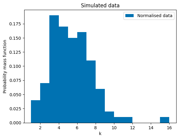
A common type of distribution found in astrophysics is a Poisson distribution as it a discrete distribution and photon counts are discrete. The brightness of high energy sources can be described with a Poisson distribution, so for this example we will use a Poisson distribution to determine the average brightness of a pulsar. We will use the following equation:
\begin{equation*} P\left( k \right) = \frac{{e^{ - \lambda } \lambda ^k }}{{k!}} \end{equation*}
Here \(\lambda\) is the expected rate of occurrences and \(k\) is the number of occurrences. In this example we choose a flat/uniform prior, which means that we assume all \(\lambda\) values are equally likely. This is done for simplicity of the example, more complicated priors will be explained in Chapter 5.
[14]:
import numpy as np
import matplotlib.pyplot as plt
from scipy.special import factorial
plt.style.use("seaborn-v0_8-colorblind")

# True mean photon count rate (λ) of the light source
true_lambda = 5# True photon count rate (per unit time)
num_observations = 100  # Number of time intervals
np.random.seed(12169)

# Simulate photon counts using a Poisson distribution
observed_counts = np.random.poisson(lam=true_lambda, size=num_observations)
total_observed_counts = np.sum(observed_counts)  # Total photon counts

plt.hist(observed_counts, 15, density=True, label="Normalised data")
plt.title("Simulated data")
plt.xlabel("k")
plt.ylabel("Probability mass function")
plt.legend()
plt.show()


# -------------------- Step 1: Define Prior  --------------------

lambda_coarse_grid = np.linspace(0, 10, 50)  # Possible λ values between 0.1 and 15

# Assume all λ values are equally likely
prior = np.ones_like(lambda_coarse_grid)  # Flat prior
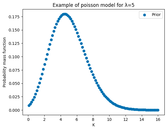
The statistical model will be a Poisson likelihood. We will use the log-likelihood, because we will work with calculations small values. The coarse grid will here be used to calculated all the likelihoods for parameter \(\lambda\).
[15]:
# -------------------- Step 2: Define model and Likelihood --------------------
def poisson_pmf(k, lam):
    return (lam**k * np.exp(-lam)) / factorial(k)

k = np.linspace(0.1, 16, 100)

plt.scatter(k, poisson_pmf(k, 5), label="Prior",alpha=1)
plt.title("Example of poisson model for λ=5")
plt.xlabel("K")
plt.ylabel("Probability mass function")
plt.legend()
plt.show()

def log_likelihood_poisson(lam, observed):
    return (np.sum(-lam +np.log(lam)*observed -np.log(factorial(observed)) ))


#Compute log-likelihood for each λ value in the grid
log_likelihoods = np.array([log_likelihood_poisson(lam, observed_counts) for lam in lambda_coarse_grid])
C:\Users\marab\AppData\Local\Temp\ipykernel_10012\3881526062.py:15: RuntimeWarning: divide by zero encountered in log
  return (np.sum(-lam +np.log(lam)*observed -np.log(factorial(observed)) ))
[16]:
# -------------------- Step 3: Define posterior probability --------------------
#Posterior ∝ Prior × Likelihood
log_posterior_unnormalized = log_likelihoods + np.log(prior)

# Normalize the posterior
log_posterior_normalized = log_posterior_unnormalized - np.max(log_posterior_unnormalized)
posterior = np.exp(log_posterior_normalized)

# MAP (Maximum A Posteriori) estimate
map_index = np.argmax(posterior)
map_lambda = lambda_coarse_grid[map_index]

plt.scatter(lambda_coarse_grid, posterior, label="Posterior", alpha=0.5)
plt.axvline(map_lambda, color="r", linestyle="--", label=f"MAP estimate: λ={map_lambda:.2f}")
plt.axvline(5, color="black", linestyle="--", label="True Value of λ")
plt.title("Posterior Distribution of λ ")
plt.xlabel("λ ")
plt.ylabel("Posterior Probability")
plt.legend()

plt.show()
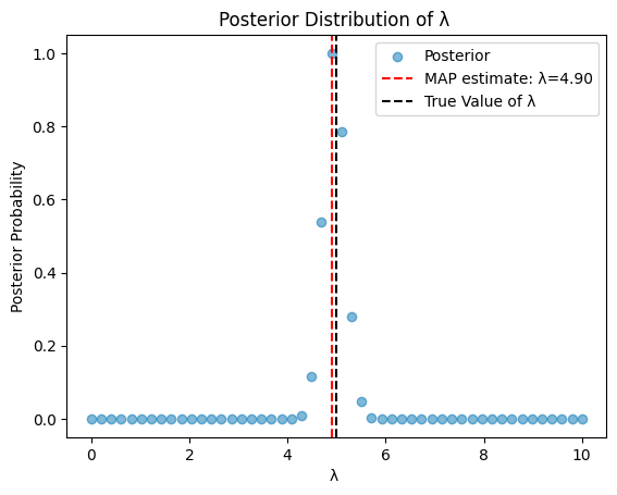
The posterior that is calculated here can now be used to slim down the ranges of possible values of the unknown parameters. Then a finer grid will be made and a new posterior will be calculated and the maximum posterior estimate will be found, which is our best fit for the parameter \(\lambda\).
[17]:
lambda_fine_grid = np.linspace(4, 6, 100)

#Repeating the steps of Bayesian inference
prior_fine = np.ones_like(lambda_fine_grid)

log_likelihoods_fine = np.array([log_likelihood_poisson(lam, observed_counts) for lam in lambda_fine_grid])

log_posterior_unnormalized_fine = log_likelihoods_fine + np.log(prior_fine)

log_posterior_normalized_fine = log_posterior_unnormalized_fine - np.max(log_posterior_unnormalized_fine)
posterior_fine = np.exp(log_posterior_normalized_fine)

map_index_fine = np.argmax(posterior_fine)
map_lambda_fine = lambda_fine_grid[map_index_fine]

#Plot results
plt.figure(figsize=(20,15))
plt.subplot(2,2,1)
plt.plot(lambda_fine_grid, prior_fine, label="Prior", alpha=1)
plt.plot(np.linspace(3,4,100),np.zeros(100), c="tab:blue")
plt.plot(np.linspace(6,7,100),np.zeros(100), c="tab:blue")
plt.vlines(4, ymin=0,ymax=1)
plt.vlines(6, ymin=0,ymax=1)
plt.title("Prior Distribution of λ ")
plt.xlabel("λ ")
plt.ylabel("Prior")
plt.legend()
plt.xlim(3,7)
plt.ylim(-0.1,1.1)


plt.subplot(2,2,2)
plt.scatter(lambda_fine_grid, np.exp(log_likelihoods_fine), label="Likelihood", alpha=1)
#plt.axvline(5, color="magenta", linestyle="--", label="True Value of λ")
plt.title("Likelihoods of λ grid ")
plt.xlabel("λ ")
plt.ylabel("Likelihood")
plt.legend()


plt.subplot(2,2,3)
plt.scatter(lambda_fine_grid, posterior_fine, label="Posterior", alpha=1)
plt.axvline(map_lambda_fine, color="r", linestyle="--", label=f"MAP estimate: λ={map_lambda_fine:.2f}")
plt.axvline(5, color="black", linestyle="--", label="True Value of λ")
plt.title("Posterior Distribution of λ ")
plt.xlabel("λ ")
plt.ylabel("Posterior Probability")
plt.legend()

plt.show()
print(f"MAP estimate of λ, so the best fit for λ: {map_lambda_fine:.2f}")
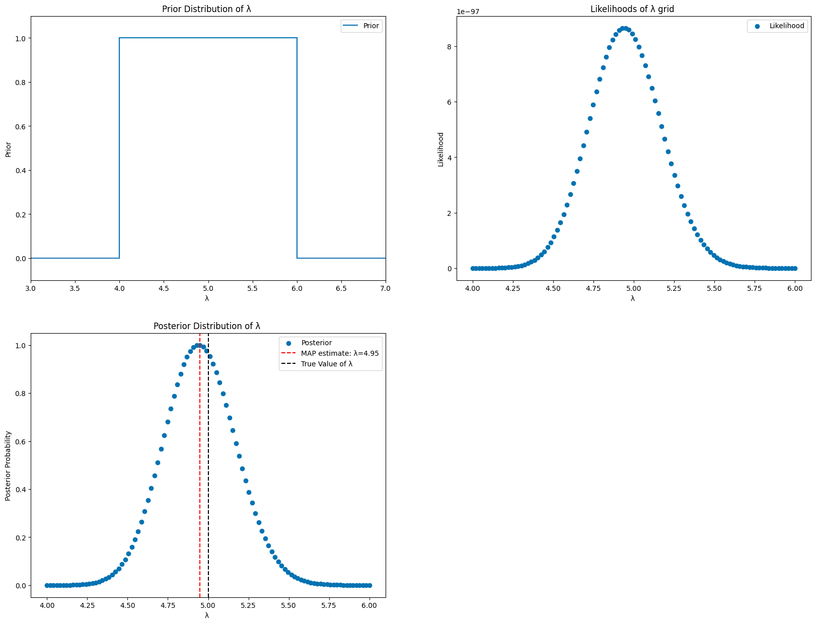
MAP estimate of λ, so the best fit for λ: 4.95
Now as we have a best fit, we can find a confidence interval on it. We can also improve our posterior if we have additional data. How to do all this will now be explained.
Computation of confidence intervals using a grid search in combination with an updated posterior
Computing confidence intervals using a grid search is a method particularly useful when analytic solutions are unavailable. By evaluating the parameter space, calculating posterior probabilities for every point and deriving credible intervals, we get a confidence interval given the data and prior knowledge such that P[Θ ∈ I | X] = 1 - \(\alpha\) where \(\alpha\) is our confidence level. In this manner it is an analogue to a frequentist confidence interval.
By first creating a fine grid of plausible values for our parameters and defining a posterior, following bayesian inference, we can compute the value of the posterior in each point. Meaning that every combination of n parameters is used to calculate the posterior giving a hypercube filled with \(m_1 \cdot m_2 \cdot ... \cdot m_n\) points (for \(m_i\) the total number of chosen grid values).
To identify the confidence interval we have two main methods. The equal tail methods consists of looking at the interval [θ(α/2),θ(1−α/2)], which determines the region where all points lay such that the probability for a point to lay in this interval is 1- \(\alpha\). This reflects the true probability the value of our parameter lies in that interval. However, this brings some ambiguity into play. Imagine a simple gaussian distribution. We can construct an \(\alpha\) = 0.5 interval on the left side going from -inf to the mean or an interval on the right side. We can also have the mean in the middle of the interval and symmetrically go to both sides. To solve this ambivalence we try to minimize the length of the interval. Or let the interval be determined by equalling the excluded area on both tail-ends.
Updating posteriors is what we do when new data is found and this will be done in the next example. When going through the steps of Bayesian inference with the new data, the old data can also be used to further improve the posterior, as was explained in the beginning of the chapter. If \(\mathcal{L}_1\) is the likelihood of the old data and \(\mathcal{L}_2\) it of the new, the likelihoods of the new and old data can be multiplied like so:
\begin{equation*} p ( \theta | y , x) \propto p ( \theta | x) \cdot \mathcal{L}_1 (y_1 | \theta , x) \cdot \mathcal{L}_2 (y_2 | \theta , x) \end{equation*}
In general for multiple old and new data sets:
\begin{equation*} \mathcal{L}_{tot} (y_1, … ,y_n | \theta , x) = \prod_{i=1}^{n} \mathcal{L} (y_i | \theta , x) \end{equation*}
Which transforms equation 4.1 into:
\begin{equation*} p ( \theta | y , x) \propto p ( \theta | x) \cdot \mathcal{L}_{tot} (y_1, … ,y_n | \theta , x) \end{equation*}
So here the prior knowledge gets used to inform the posterior probability.
Complete example
To illustrate Bayesian inference using grid searches to determine confidence intervals and updating said posterior, we will look at the intensity I\(_e\) of a galaxy at several radii. It has three parameters of which two are independent. r\(_e\) is the scale length for which the r=0 intensity has dropped to half its value, n is the Sersic index controlling the curvature of the profile and b\(_n\) is determined by solving the eq.
or for n > 0.5 the approximation:
giving the full profile the following form:
[18]:
import numpy as np
import matplotlib.pyplot as plt
import scipy.stats
from tqdm.notebook import tqdm
import numpy as np
import scipy.optimize as opt
import scipy.special as sp
import matplotlib.pyplot as plt

# -------------------- Step 1: Simulate SNR density distribution --------------------
np.random.seed(12169237)

def sersic_profile(r, r_e, n):
    """Compute the Sérsic profile"""
    b_n = 2 * n - 1/3 +4/(405*n) + 46/(25515*n**2) # Approximation for b_n
    rho = np.exp(-b_n * ((r / r_e)**(1/n) - 1))
    return rho / np.max(rho)


R_max  = 1e3
r_range = np.linspace(0,R_max,10000)

# True parameters
n = np.linspace(0.1,1, 5)
r_e = 350

plt.figure()
plt.title("Sersic Profile for r$_e$ = 350 and several n")
colors =  ['#0173b2', '#de8f05', '#029e73', '#d55e00', '#cc78bc', '#ca9161', '#fbafe4', '#949494', '#ece133', '#56b4e9']
for i in range(len(n)):
    plt.plot(r_range, sersic_profile(r_range, r_e, n[i]), label=f"n = {n[i]}", c=colors[i])

plt.xlim(0,R_max)

plt.xlabel("Radial distance (r)")
plt.ylabel("Density")
plt.legend()

plt.show()
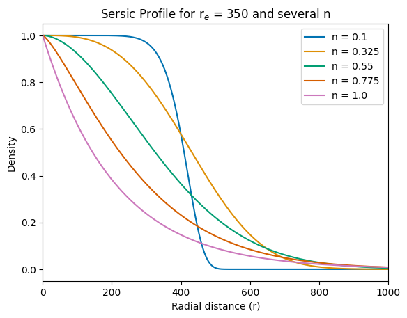
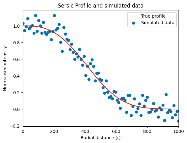
We will sample n points from this distribution (with n = 0.35, as an example, normally we have profiles ~1 or ~4), picking a relatively imprecise simulation first. We’ll do so to show how we can improve this later by updating the posterior with a new data set. And to keep things general we normalise the intensity by I\(_0\). The simulated data will be given a gaussian scatter around the true value to simulate observational uncertainties. In the plot below we can see the form of this sersic profile and the simulated set.
[19]:
def sim_data(r,r_e,n, fractional_uncertainty):
    y_true = sersic_profile(r,r_e,n)
    #y_unc_true = np.abs(y_true)*
    y_sample = np.random.normal(y_true, fractional_uncertainty, size=len(r))
    return y_sample, fractional_uncertainty#, y_unc_true


R_max  = 1e3
r_range_model = np.linspace(0,R_max,1000)

# True parameters
true_n = 0.35
true_r_e = 350

#simulating data
unc = 0.08
r_range_sim = np.linspace(0,R_max,100)

sim_r, sim_r_uncertainty = sim_data(r_range_sim, true_r_e , true_n, unc)
#
plt.figure()
plt.title("Sersic Profile and simulated data")
plt.plot(r_range_model, sersic_profile(r_range_model, true_r_e, true_n), c="red", label="True profile")
plt.scatter(r_range_sim, sim_r, alpha=1, label="Simulated data")
plt.xlim(0,R_max)
plt.xlabel("Radial distance (r)")
plt.ylabel("Normalised intensity")
plt.legend()
plt.show()
After simulating the data we can start the Bayesian inference. We start with choosing a prior. For now we will assume a flat prior which is around the true n and true r\(_e\) value. From looking at different simulated sersic profiles such bounds could in practise be estimated. The statistical model will be a Gaussian likelihood. Since we will work with calculations with small values we prefer the log-likelihood to reduce numerical problems.
Calculating the posterior then comes down to calculating the product of the prior and likelihood (or the exponent containing the sum of the log-prior and the log-likelihood).
[20]:
# -------------------- Step 2: Define Prior and Likelihood --------------------
def flat_prior(n, r_e ):
    if 0.1<= n <= 0.6 and 200 <= r_e <= 500:  # Example bounds
        return 1
    return 0

def log_likelihood(r, observed, sigma, r_e, n,):
    model_density = sersic_profile(r, r_e, n)
    return (-np.sum(0.5 * ((observed - model_density) / sigma) ** 2 + np.log(sigma * np.sqrt(2 * np.pi))))

def posterior(n_space, r_e_space, r_range, sim_r, sim_r_uncertainty, prior):
    log_posterior_grid = np.full((len(n_space),len(r_e_space)), -np.inf)

    # Loop over all combinations of n and r_e, filling in the grid with values of the posterior
    for i in tqdm(range(len(n_space))):
        for j in range(len(r_e_space)):
            prior_val = prior(n_space[i],r_e_space[j] )
            if prior_val == 0:
                continue
            else:
                # Compute likelihood for this position (using the simulated data)
                # Compute the posterior for this position,
                # i represents the n parameter (axis = 0), and j represents the r_e parameter (axis=1)
                log_likelihood_value = log_likelihood(r_range, sim_r, sim_r_uncertainty,r_e_space[j], n_space[i] )
                log_posterior_grid[i, j] = log_likelihood_value + np.log(prior_val)

    posterior = np.exp(log_posterior_grid - np.max(log_posterior_grid))

    return  posterior
Using a grid search allows us to calculate this posterior for every point in the grid, as explained above. We will first compute a coarse grid to determine the range of values without spending excess time on computing fine grids in unwanted regions.
[21]:
# Create a "coarse" 2D grid of r_e and n,
#simulation time = 10 seconds
n_space = np.linspace(0.2, 0.6, 250)
r_e_space = np.linspace(200, 500, 250)
posterior_grid = posterior(n_space, r_e_space, r_range_sim, sim_r, sim_r_uncertainty, flat_prior)
posterior_grid /= np.sum(posterior_grid)  # Normalizing the grid
[22]:
#  best-fit parameters found by using argmax and indexing
max_idx = np.unravel_index(np.argmax(posterior_grid), posterior_grid.shape)
best_fit_n = n_space[max_idx[0]]
best_fit_r_e = r_e_space[max_idx[1]]

print(f"Best-fit n: {best_fit_n:.3f}")
print(f"Best-fit r_e: {best_fit_r_e:.3f}")
Best-fit n: 0.338
Best-fit r_e: 348.193
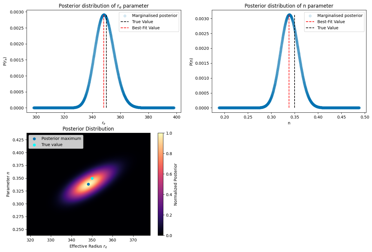
To get a feeling of how the posterior distribution of both parameters looks like we will plot the following:
A 2D posterior density
The marginalised posterior for r\(_e\)
The marginalised posterior for n
This gives us a feeling for how the distribution looks like, enabling us to determine a finer grid.
Marginalising over one of the parameters is done by summing (for continuous function an integral is taken) over all other parameters, collapsing the posterior into a single-parameter function.
We then plot all of these, along with the best fit value and the true values.
[23]:
P_r_e = np.sum(posterior_grid, axis=0)
P_n = np.sum(posterior_grid, axis=1)

#normalisation
P_r_e  /= np.sum(P_r_e )
P_n /= np.sum(P_n)


plt.figure(figsize=(15,10))
plt.subplot(2,2,1)
plt.title("Posterior distribution of r$_e$ parameter")
plt.scatter(r_e_space, P_r_e, label="Marginalised posterior", alpha=0.5)
plt.vlines(true_r_e, ymin=np.min(P_r_e),ymax=np.max(P_r_e), color="black", linestyles="--", label="True Value")
plt.vlines(x= best_fit_r_e, ymin=np.min(P_r_e),ymax=np.max(P_r_e), color="r", linestyles="--", label="Best-Fit Value")
plt.xlabel("$r_e$")
plt.ylabel("P($r_e$)")
plt.legend()

plt.subplot(2,2,2)
plt.title("Posterior distribution of n parameter")
plt.scatter(n_space,P_n,  label="Marginalised posterior", alpha=0.5)
plt.vlines(x= best_fit_n,ymin=np.min(P_n),ymax=np.max(P_n), color="r", linestyles="--", label="Best-Fit Value")
plt.vlines(true_n, ymin=np.min(P_n),ymax=np.max(P_n), color="black", linestyles="--", label="True Value")
plt.xlabel("n")
plt.ylabel("P(n)")
plt.legend()


plt.subplot(2,2,3)
plt.imshow(posterior_grid, extent=[r_e_space.min(), r_e_space.max(), n_space.min(), n_space.max()], origin='lower', aspect='auto', cmap='magma')
plt.colorbar(label="Normalized Posterior",cmap='magma' )
plt.scatter(best_fit_r_e, best_fit_n, label="Posterior maximum")
plt.scatter(true_r_e,true_n, label="True value",c="cyan")
plt.title("Posterior Distribution")
plt.xlabel("Effective Radius $r_e$")
plt.ylabel("Parameter $n$")
plt.ylim(best_fit_n-0.1, best_fit_n+0.1)
plt.xlim(best_fit_r_e-30, best_fit_r_e+30)
plt.legend(loc="upper left")
plt.show()

We can see that both the marginalised posteriors have Gaussian-like curves relatively close to the true parameters. We can now create a smaller and finer grid to correctly determine the confidence intervals of both parameters, which we, until this point, have neglected. We center the grid around the best fit value and add many more points to the grid. Then in the same manner we plot the (marginalised) posterior. This will in principle have the same shape as above, but with many more points so that the intervals between points is smaller than the wanted precision.
[24]:
#defining a finer grid. Not this well take >1min of computing time
n_space = np.linspace(best_fit_n-0.15, best_fit_n+0.15, 2000)
r_e_space = np.linspace(best_fit_r_e-50, best_fit_r_e+50, 2000)
posterior_grid = posterior(n_space, r_e_space, r_range_sim, sim_r, sim_r_uncertainty, flat_prior)
P_r_e = np.sum(posterior_grid, axis=0)
P_n = np.sum(posterior_grid, axis=1)
P_r_e  /= np.sum(P_r_e )
P_n /= np.sum(P_n)
[25]:
plt.figure(figsize=(15,10))
plt.subplot(2,2,1)
plt.title("Posterior distribution of r$_e$ parameter")
plt.scatter(r_e_space, P_r_e, label="Marginalised posterior", alpha=0.15)
plt.vlines(true_r_e, ymin=np.min(P_r_e),ymax=np.max(P_r_e), color="black", linestyles="--", label="True Value")
plt.vlines(x= best_fit_r_e, ymin=np.min(P_r_e),ymax=np.max(P_r_e), color="r", linestyles="--", label="Best-Fit Value")
plt.xlabel("$r_e$")
plt.ylabel("P($r_e$)")
plt.legend()

plt.subplot(2,2,2)
plt.title("Posterior distribution of n parameter")
plt.scatter(n_space,P_n,  label="Marginalised posterior", alpha=0.15)
plt.vlines(x= best_fit_n,ymin=np.min(P_n),ymax=np.max(P_n), color="r", linestyles="--", label="Best-Fit Value")
plt.vlines(true_n, ymin=np.min(P_n),ymax=np.max(P_n), color="black", linestyles="--", label="True Value")
plt.xlabel("n")
plt.ylabel("P(n)")
plt.legend()


plt.subplot(2,2,3)
plt.imshow(posterior_grid, extent=[r_e_space.min(), r_e_space.max(), n_space.min(), n_space.max()], origin='lower', aspect='auto', cmap='magma')
plt.colorbar(label="Normalized Posterior",cmap='magma' )
plt.scatter(best_fit_r_e, best_fit_n, label="Posterior maximum")
plt.scatter(true_r_e,true_n, label="True value",c="cyan")
plt.title("Posterior Distribution")
plt.xlabel("Effective Radius $r_e$")
plt.ylabel("Parameter $n$")
plt.ylim(best_fit_n-0.1, best_fit_n+0.1)
plt.xlim(best_fit_r_e-30, best_fit_r_e+30)
plt.legend(loc="upper left")
plt.show()
[26]:
#  best-fit parameters
max_idx = np.unravel_index(np.argmax(posterior_grid), posterior_grid.shape)
best_fit_n = n_space[max_idx[0]]
best_fit_r_e = r_e_space[max_idx[1]]
print(f"Best-fit n: {best_fit_n:.3f}")
print(f"Best-fit r_e: {best_fit_r_e:.3f}")
Best-fit n: 0.338
Best-fit r_e: 348.268
Confidence intervals
Up until now, everything is similar as in the previous example. We now also want to say something about the confidence interval around the best fit value. To do so we will compute the cumulative distribution of the posterior. This is the probability for a random variable X to take on a value less than or equal to a certain value x. The CDF can then be used to find the percentile forming the interval’s bounds. These percentiles are combined with the sample statistic, enabling to define the interval in the parameter space.
The first function will do so by looking for exactly these boundaries. It will work for most applications. In the case we have a probability distribution that has two maxima or is centered around a hard bound (lets say the number of particles which can never be 0 but a distribution that goes into the negatives), we can use the second function. It works similarly as the first function but will calculate the probability to lie within two bounds, {i,j}, of the parameter space using a CDF. When this matches the desired confidence interval, these bounds are saved. We then search for all ambiguous boundaries also having such valid interval and minimize it to obtain the one with minimum width. This will provide the wanted interval.
Since we will be working with a one bell curve distribution which does not have strict bounds, we will show of both work and give the same result and then omit the second approach for the rest of the example.
[27]:
def compute_equal_tailed_interval(parameter_space, posterior, alpha):
    cdf = np.cumsum(posterior)
    lower_bound = parameter_space[np.searchsorted(cdf, alpha / 2)]
    upper_bound = parameter_space[np.searchsorted(cdf, 1 - alpha / 2)]
    return lower_bound, upper_bound

def find_minimal_interval(parameter_space, posterior, alpha):
    # Normalize posterior to ensure it sums to 1
    posterior = posterior / np.sum(posterior)

    # Initialize variables
    min_width = np.inf
    best_interval = None
    target_prob =  1-alpha

    # Sliding window
    for i in tqdm(range(len(parameter_space)), desc="Parameter space"):  # Start of the window
        cumulative_prob = 0  # Reset cumulative probability for each new starting point

        for j in range(i, len(parameter_space)):  # End of the window
            # Expand the window by adding the probability at j
            cumulative_prob += posterior[j]

            # Check if the window meets or exceeds the target probability
            if cumulative_prob >= target_prob:
                # Calculate the width of the current window
                width = parameter_space[j] - parameter_space[i]

                # If the current window's width is smaller, update the best interval
                if width < min_width:
                    min_width = width
                    best_interval = (round(parameter_space[i], 3), round(parameter_space[j], 3))

                # No need to continue further as we want to minimize the width
                break  # Move to the next starting point (i)

    return best_interval
[28]:
P_r_e = np.sum(posterior_grid, axis=0)
P_n = np.sum(posterior_grid, axis=1)

# Normalize the marginalized distributions
n_mag = P_n /  np.sum(P_n)
r_e_mag = P_r_e /  np.sum(P_r_e)

# Compute confidence intervals (# 68% confidence)
alpha = 0.16
n_lower, n_upper = compute_equal_tailed_interval(n_space, n_mag, alpha)
r_e_lower, r_e_upper = compute_equal_tailed_interval(r_e_space, r_e_mag, alpha)
# Find minimal-width intervals for n and r_e
n_min_interval = find_minimal_interval(n_space, n_mag, alpha)
r_e_min_interval = find_minimal_interval(r_e_space, r_e_mag, alpha)
[29]:
plt.figure(figsize=(15, 10))

# Marginalized n
plt.subplot(2, 2, 1)
plt.plot(n_space, n_mag, label='P(n)')
plt.title("CDF n equal tail")
plt.axvline(n_lower, color='green', linestyle='--', label="Confidence interval")
plt.axvline(n_upper, color='green', linestyle='--')
plt.axvline(true_n, color='black', linestyle='--')
plt.xlim(0.25,0.45)
plt.xlabel("n")
plt.ylabel("Posterior Probability")
plt.legend()

plt.subplot(2, 2, 3)
plt.plot(n_space, n_mag, label='P(n)')
plt.title("CDF n window")
plt.axvline(n_min_interval[0], color='green', linestyle='--', label="Confidence interval")
plt.axvline(n_min_interval[1], color='green', linestyle='--')
plt.axvline(true_n, color='black', linestyle='--')
plt.xlim(0.25,0.45)
plt.xlabel("n")
plt.ylabel("Posterior Probability")
plt.legend()

# Marginalized r_e
plt.subplot(2, 2, 2)
plt.title("CDF $r_e$ equal tail")
plt.plot(r_e_space, r_e_mag, label=r'$P(r_e)$')
plt.axvline(r_e_lower, color='green', linestyle='--', label="Confidence interval")
plt.axvline(r_e_upper, color='green', linestyle='--')
plt.axvline(true_r_e, color='black', linestyle='--')
plt.xlim(320,380)
plt.xlabel(r"$r_e$")
plt.ylabel("Posterior Probability")
plt.legend()

plt.subplot(2, 2, 4)
plt.title("CDF $r_e$ window")
plt.plot(r_e_space, r_e_mag, label=r'$P(r_e)$')
plt.axvline(r_e_min_interval[0], color='green', linestyle='--', label="Confidence interval")
plt.axvline(r_e_min_interval[1], color='green', linestyle='--')
plt.axvline(true_r_e, color='black', linestyle='--', label="True Value")
plt.xlabel(r"$r_e$")
plt.ylabel("Posterior Probability")
plt.legend()
plt.xlim(320,380)
plt.tight_layout()
plt.show()

[30]:
from IPython.display import display, Math, Markdown #module to properly show intervals

#But it is more insightful to view the upper and lower bounds with respect to the best fit value
display( Markdown(r"Best fit value for n with confidence interval:"), Math(f"{best_fit_n:.2f}^{{+{-(best_fit_n-n_upper):.2f}}}_{{-{best_fit_n - n_lower:.2f}}}"))

display( Markdown(r"Best fit value for r_e with confidence interval:"), Math(f" {best_fit_r_e:.0f}^{{+{-(best_fit_r_e-r_e_upper):.0f}}}_{{-{best_fit_r_e - r_e_lower:.0f}}}"))
Best fit value for n with confidence interval:
Best fit value for r_e with confidence interval:
In the plots above we see the calculated intervals, which are very similar for both approaches. We can also see the true values lies within the 1 \(\sigma\) interval for both parameters. In principle one is done. We have to the best of our ability calculated a best-fit value with confidence intervals for the provided data.
However, to show how updating of the posterior works we go one step further. Imagine the case where you do a second study on the luminosity of the galaxy and obtain 200 instead of 100 data points with an even smaller uncertainty (0.05 to 0.08) from a newer telescope. We could argue the previous data is still pretty useful. To see how we can use this “old” data we simulate the newer data and just like above calculate it’s posterior grid, find the confidence interval and its most probable value. However, we calculate two posteriors this time. One where we omit the previous data and one where we “update” it with this data.
Before running the code in the cells below, think of what you expect of the new data set and whether the old data can have a significant effect/ constrains the parameter space noticeably.
[31]:
unc_better = 0.06
r_range_better = np.linspace(0,R_max,150)

sim_r_2, sim_r_uncertainty_2 = sim_data(r_range_better, true_r_e, true_n, unc_better)

plt.figure(figsize=(10,5))
plt.subplot(1,2,1)
plt.title("First data set")
plt.plot(r_range_model, sersic_profile(r_range_model, true_r_e, true_n),c="red",label="True model")
plt.scatter(r_range_sim, sim_r, alpha=0.5, c="tab:blue",label="Data")
plt.xlim(0,R_max)
plt.xlabel("Radial distance (r)")
plt.ylabel("Normalised intensity")
plt.legend()

plt.subplot(1,2,2)
plt.title("Second data set")
plt.plot(r_range_model, sersic_profile(r_range_model, true_r_e, true_n), c="red", label="True model")
plt.scatter(r_range_better, sim_r_2, alpha=0.5, c="tab:blue", label="Data")
plt.xlim(0,R_max)
plt.xlabel("Radial distance (r)")
plt.ylabel("Normalised intensity")
plt.legend()

plt.show()

[32]:
#calculating the posterior for the second data set (again computation time ~1.5min)
posterior_grid_2 = posterior(n_space, r_e_space, r_range_better, sim_r_2, sim_r_uncertainty_2, flat_prior)
[33]:
#normalizing the posterior
posterior_grid_2 /= np.sum(posterior_grid_2)

#Posterior update with the original posterior grid and normalisation of it.
posterior_grid_updated = posterior_grid_2 * posterior_grid
posterior_grid_updated /= np.sum(posterior_grid_updated)

#best-fit parameters
max_idx = np.unravel_index(np.argmax(posterior_grid_2), posterior_grid_2.shape)
best_fit_n_2 = n_space[max_idx[0]]
best_fit_r_e_2 = r_e_space[max_idx[1]]

print(f"Best-fit n: {best_fit_n_2:.3f}")
print(f"Best-fit r_e: {best_fit_r_e_2:.3f}")

max_idx = np.unravel_index(np.argmax(posterior_grid_updated), posterior_grid_updated.shape)
best_fit_n_updated = n_space[max_idx[0]]
best_fit_r_e_updated = r_e_space[max_idx[1]]
print('\n')
print(f"Best-fit n with update: {best_fit_n_updated:.3f}")
print(f"Best-fit r_e with update: {best_fit_r_e_updated:.3f}")
Best-fit n: 0.356
Best-fit r_e: 348.718


Best-fit n with update: 0.351
Best-fit r_e with update: 348.568
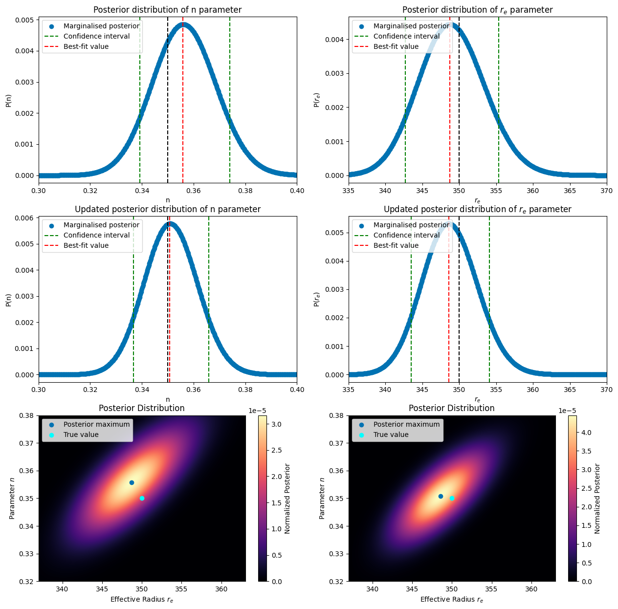
We can already see the best fit value for the updated posterior is more accurate than the one without update. Let’s see how the confidence intervals are influenced. To do so we again will plot the marginalised posterior and the density plot as above.
[34]:
P_r_e_2 = np.sum(posterior_grid_2, axis=0)
r_e_mag_2 = P_r_e_2 / np.sum(P_r_e_2)
P_n_2 = np.sum(posterior_grid_2, axis=1)
n_mag_2 = P_n_2 / np.sum(P_n_2)

P_r_e_updated = np.sum(posterior_grid_updated, axis=0)
r_e_mag_updated = P_r_e_updated / np.sum(P_r_e_updated)
P_n_updated = np.sum(posterior_grid_updated, axis=1)
n_mag_updated = P_n_updated / np.sum(P_n_updated)


alpha = 0.16
# Compute confidence intervals
n_lower_2, n_upper_2 = compute_equal_tailed_interval(n_space, n_mag_2, alpha)
r_e_lower_2, r_e_upper_2 = compute_equal_tailed_interval(r_e_space, r_e_mag_2, alpha)

n_lower_updated, n_upper_updated = compute_equal_tailed_interval(n_space, n_mag_updated, alpha)
r_e_lower_updated, r_e_upper_updated = compute_equal_tailed_interval(r_e_space, r_e_mag_updated, alpha)


plt.figure(figsize=(15,15))
plt.subplot(3,2,2)
plt.title("Posterior distribution of $r_e$ parameter")
plt.scatter(r_e_space, P_r_e_2, label="Marginalised posterior")
plt.axvline(r_e_lower_2, color='green', linestyle='--', label="Confidence interval")
plt.axvline(r_e_upper_2, color='green', linestyle='--')
plt.axvline(best_fit_r_e_2, color="r", linestyle="--", label="Best-fit value")
plt.axvline(true_r_e, color='black', linestyle='--')
plt.xlabel("$r_e$")
plt.legend(loc="upper left")
plt.ylabel("P($r_e$)")
plt.xlim(335, 370)

plt.subplot(3,2,1)
plt.title("Posterior distribution of n parameter")
plt.scatter(n_space,P_n_2, label="Marginalised posterior")
plt.axvline(n_lower_2, color='green', linestyle='--', label="Confidence interval")
plt.axvline(n_upper_2, color='green', linestyle='--')
plt.axvline(best_fit_n_2, color="r", linestyle="--", label="Best-fit value")
plt.legend(loc="upper left")
plt.axvline(true_n, color='black', linestyle='--')

plt.xlabel("n")
plt.ylabel("P(n)")
plt.xlim(0.3, 0.4)

plt.subplot(3,2,4)
plt.title("Updated posterior distribution of $r_e$ parameter")
plt.scatter(r_e_space, P_r_e_updated,label="Marginalised posterior")
plt.axvline(r_e_lower_updated, color='green', linestyle='--',label="Confidence interval")
plt.axvline(r_e_upper_updated, color='green', linestyle='--')
plt.axvline(x= best_fit_r_e_updated, color="red", linestyle="--", label="Best-fit value")
plt.axvline(true_r_e, color='black', linestyle='--')
plt.xlabel("$r_e$")
plt.legend(loc="upper left")
plt.ylabel("P($r_e$)")
plt.xlim(335, 370)


plt.subplot(3,2,3)
plt.title("Updated posterior distribution of n parameter")
plt.scatter(n_space,P_n_updated, label="Marginalised posterior")
plt.axvline(n_lower_updated, color='green', linestyle='--', label="Confidence interval")
plt.axvline(n_upper_updated, color='green', linestyle='--')
plt.axvline(x= best_fit_n_updated, color="red", linestyle="--", label="Best-fit value")
plt.axvline(true_n, color='black', linestyle='--')
plt.legend(loc="upper left")
plt.xlabel("n")
plt.ylabel("P(n)")
plt.xlim(0.3, 0.4)


plt.subplot(3,2,5)
plt.title("Posterior grid of second data set")
plt.imshow(posterior_grid_2, extent=[r_e_space.min(), r_e_space.max(), n_space.min(), n_space.max()], origin='lower', aspect='auto', cmap='magma')
plt.colorbar(label="Normalized Posterior",cmap='magma' )
plt.scatter(best_fit_r_e_2, best_fit_n_2, label="Posterior maximum")
plt.scatter(true_r_e,true_n, label="True value", c="cyan")
plt.title("Posterior Distribution")
plt.xlabel("Effective Radius $r_e$")
plt.ylabel("Parameter $n$")
plt.ylim(true_n-0.03, true_n+0.03)
plt.xlim(true_r_e-13, true_r_e+13)
plt.legend(loc="upper left")

plt.subplot(3,2,6)
plt.title("Updated posterior grid")
plt.imshow(posterior_grid_updated, extent=[r_e_space.min(), r_e_space.max(), n_space.min(), n_space.max()], origin='lower', aspect='auto', cmap='magma')
plt.colorbar(label="Normalized Posterior",cmap='magma' )
plt.scatter(best_fit_r_e_updated, best_fit_n_updated, label="Posterior maximum")
plt.scatter(true_r_e,true_n, label="True value", c="cyan")

plt.title("Posterior Distribution")
plt.xlabel("Effective Radius $r_e$")
plt.ylabel("Parameter $n$")
plt.ylim(true_n-0.03, true_n+0.03)
plt.xlim(true_r_e-13, true_r_e+13)
plt.legend(loc="upper left")
plt.show()
[35]:
# Data formatting for the  pretty table to have overview of found values
from IPython.display import display, Markdown

data = [
    ["Posterior", "Best Fit n with Confidence Interval", "Best Fit $r_e$ with Confidence Interval"],
    ["1",
     f"$ {best_fit_n:.2f}^{{+{n_upper - best_fit_n:.2f}}}_{{-{best_fit_n - n_lower:.2f}}} $",
     f"$ {best_fit_r_e:.0f}^{{+{r_e_upper - best_fit_r_e:.0f}}}_{{-{best_fit_r_e - r_e_lower:.0f}}} $"
    ],
    ["2",
     f"$ {best_fit_n_2:.2f}^{{+{n_upper_2 - best_fit_n_2:.2f}}}_{{-{best_fit_n_2 - n_lower_2:.2f}}} $",
     f"$ {best_fit_r_e_2:.0f}^{{+{r_e_upper_2 - best_fit_r_e_2:.0f}}}_{{-{best_fit_r_e_2 - r_e_lower_2:.0f}}} $"
    ],
    ["Updated",
     f"$ {best_fit_n_updated:.2f}^{{+{n_upper_updated - best_fit_n_updated:.2f}}}_{{-{best_fit_n_updated - n_lower_updated:.2f}}} $",
     f"$ {best_fit_r_e_updated:.0f}^{{+{r_e_upper_updated - best_fit_r_e_updated:.0f}}}_{{-{best_fit_r_e_updated - r_e_lower_updated:.0f}}} $"
    ]
]

# Construct the Markdown table
table_markdown = "| " + " | ".join(data[0]) + " |\n"
table_markdown += "| " + " | ".join(["---"] * len(data[0])) + " |\n"
for row in data[1:]:
    table_markdown += "| " + " | ".join(row) + " |\n"

# Display the table
display(Markdown(table_markdown))
Posterior |
Best Fit n with Confidence Interval |
Best Fit \(r_e\) with Confidence Interval |
|---|---|---|
1 |
$ 0.34^{+0.03}_{-0.03} $ |
$ 348^{+10}_{-9} $ |
2 |
$ 0.36^{+0.02}_{-0.02} $ |
$ 349^{+7}_{-6} $ |
Updated |
$ 0.35^{+0.02}_{-0.01} $ |
$ 349^{+6}_{-5} $ |
We can see that the updated case both has a more accurate value (closer to the true value) and has more precision (smaller confidence interval). For this scenario we can thus conclude that the update made sense. If for example your newer data set was way less uncertain or had an order of magnitude more points, the effects would have been less. Updating it in this case might even make it worse compared to only using the “better” data.
Conclusions
In conclusion, we see that using Bayesian inference is an appropriate method to obtain parameters from a multi-variable model. Using a grid to do so is computationally intense but does work. In Chapter 6 we will discuss a more efficient method. Obtaining the confidence intervals from the CDF is in turn a reliable approach to get a grip on the precision acquired from the data. The two methods shown work in principle both but have their own niche place, which is dependent on the type of data one has. We see the more data points with a smaller inherent uncertainty results in better final results and that updating your posterior with previous data could further help out your precision and accuracy.
References
Ciotti, L. & Bertin, G., 1999, arXiv:astro-ph/9911078
Eadie, G.M., Speagle, J.S., Cisewski-Kehe, J., 2023, arXiv:2302.04703
Graham, A.W. & Driver, S.P., 2005, Publications of the Astronomical Society of Australia, 22