Chapter 2: Information Criterions and Bootstrap Confidence Intervals
In this chapter, we’ll cover the Akaike Information Criterion (AIC) and Bayesian Information Criterion (BIC) for nested models, as well as the bootstrap method for confidence intervals.
Nested Models
Let’s say we have model A with variables \(\theta_1\), \(\theta_2\) and \(\theta_3\). Model B is nested in model A if model B contains a subset of the variables of model A, e.g. if model B has variables \(\theta_1\) and \(\theta_3\). We call model B a \(\textbf{nested model}\). Model B is \(\textbf{not}\) a nested model if it contains a variable that model A doesn’t contain, e.g. if model B has variables \(\theta_1\), \(\theta_3\) and \(\theta_4\).
Model A can be seen as the true model which describes the data. When researching, you don’t know the true model, but you can construct a model B which is a nested model of model A. In order to check if model B doesn’t include unnecessary parameters and that the model isn’t overfitting the data, the Akaike Information Criterion and the Bayesian Information Criterion can be used.
In this chapter we’ll focus on the Akaike Information Criterion and Bayesian Information criterion specifically for nested models, as working with non-nested models would require to take the different normalisation constants of the likelihoods of the models into account. This can be done of course, but explaining this concept isn’t the primary goal of this chapter and so we won’t go into this any further.
Akaike Information Criterion (AIC)
The \(\textbf{Akaike Information Criterion (AIC)}\) is an estimator of prediction error of statistical models. It is a method for evaluating how well a model fits the data it was generated from. AIC is used to compare different models and determine which model is the best fit. This best fit is the one that explains the greatest amount of variation and has the minimal amount of information loss, using the fewest amount of parameters. The equation for the AIC is as follows;
It combines the maximum likelihood \(\hat{\mathcal{L}}\) and the number of parameters \(p_k\). The best model will give the lowest value. From Eq. 2.1 you can see that the AIC discourages overfitting. By adding more parameters, the AIC value will increase. The goodness of the fit, determined with the max-likelihood, will help decrease the AIC score.
Note: The AIC gives a qualitative comparison between models, it does not say anything about the quality of the models themself. So after selecting a model with the AIC, you need to validate the quality of the model. This can be done for instance by checking the models residuals.
Simple usage of AIC values
Let \(\mathrm{AIC}_{min}\) be the minimal AIC value. The following expression can be used to compare different AIC scores (\(\mathrm{AIC}_{i}\)) with \(\mathrm{AIC}_{min}\).
This quantity \(c\) is proportional to the probability of that the model \(\mathrm{AIC}_{i}\) minimizes the information loss. Say you have three models with the following values: \(\mathrm{AIC}_1 = 101\), \(\mathrm{AIC}_2 = 104\) and \(\mathrm{AIC}_3 = 111\).
\begin{equation} c = \begin{cases} e^{\frac{101 - 104}{2}} \approx 0.223 \\ e^{\frac{101 - 111}{2}} \approx 0.007\\ \end{cases} \end{equation} This means that model 2 is 0.223 times and model 3 is 0.007 times as probable as model 1 to minimize the information loss. Depending on the selection criteria, model 3 can probably be rejected. The quantity \(c\) is known as the relative likelihood of model \(i\) and it is closely related to the likelihood ratio used in the likelihood-ratio test.
Bayesian Information Criterion (BIC)
The \(\textbf{Bayesian Information Criterion (BIC)}\) is another statistical measure used to evaluate how good of a fit a model is. As with the AIC, both unexplained variation and a higher number of variables increase the BIC value. However, in addition to the penalty for the number of parameters in the AIC, the BIC also penalises for the amount of data points n. The equation for the BIC is as follows:
where \(\hat{\mathcal{L}}\) is the maximum likelihood, \(n\) is the number of data points and \(p_k\) is the number of parameters.
One of the advantages of using the Bayesian Information Criterion is that it’s fairly simple and therefore easy to compute. Its penalty for the amount of parameters also helps preventing overfitting and using the BIC to compare models is very straightforward in general. Of course, the BIC also has its disadvantages. One important limitation to the BIC is that \(n\) has to be much larger than \(p_k\) for the expression to be valid. It also relies on assuming that the true model is one of the candidate models, and the same penalty for the number of parameters that helps prevent overfitting might also lead to oversimplification.
Let’s see a simple example of using the Bayesian Information Criterion below. We’ll compare some model A and B for a dataset of 600 data points and we assume the maximum likelihood is 0.5 for model A and 0.3 for model B. Furthermore, model A uses 3 parameters while model B uses 4.
Since we want to minimalise the BIC value, the model with the lowest BIC (model A in the example) is assumed to be a better model than the one with a higher BIC. A little disclaimer: this does not necessarily mean that the model with the lowest BIC is a good fitting model objectively, it just means it explains the data better than the other model did.
In the example above, we just assumed that the maximum likelihoods were equal to certain numbers, but normally you would need to calculate the likelihood yourself. Chapter 1 contains more information about calculating the maximum likelihood.
AIC vs BIC
Though the Akaike Information Criterion and the Bayesian Information Criterion are pretty similar, they also have their differences. As mentioned above, the AIC assumes the true model isn’t among the tested models, while the BIC assumes the true model \(\textit{is}\) among the tested models. Furthermore, the BIC penalises the complexity of the models more than the AIC does. Both of these differences lead towards the following; When \(n \rightarrow \infty\) and \(p_k < \sqrt{n}\):
AIC selects the best predictive model among a number of possibly misspecified models.
BIC selects the true model (with minimal number of necessary parameters) if it is included in the candidate set.
The example below shows the AIC plotted against the BIC. Random data is generated from the true model, in this case a polynomial with 4 parameters. For the maximum likelihood the Gaussian probability density function is used \(\hat{\mathcal{L}}= \frac{1}{\sqrt{2\pi}\sigma} e^{-\frac{(x - \mu)^2}{2\sigma^2}}\). Taking the natural logarithm together with the definition of the log likelihood function given in Chapter 1 gives the following equation for \(\ln(\hat{\mathcal{L}})\):
For simplicity the prefactor of the Gaussian function is left out in Eq. 2.4, because it is a constant.
[1]:
#IMPORTS AND FUNCTIONS
import numpy as np
from scipy.optimize import curve_fit
import matplotlib.pyplot as plt
from scipy.special import logsumexp

#The true polynomial model
true_values = [20, 3, 50, 101]
def true_model(x, a=true_values[0], b=true_values[1], c=true_values[2], d=true_values[3]):
    return a*x**3 + b*x**2 + c*x + d

#Function to generate different degrees of polynomial functions
def poly_model(x, *p):
    return  np.polyval(p, x)

#Function to simulate data using the true model
def sim_data(x, uncertainty=0.2):
    y_true = model(x)
    y_unc_true = np.abs(y_true)*uncertainty
    y_sample = np.random.normal(y_true, y_unc_true, size=len(x))
    return y_sample, y_unc_true

#The likelihood function assuming it is a Gaussian distribution
def log_gaussian_likelihood(model, y, y_err):
    L = np.sum(-0.5*((model-y)**2)/y_err**2)
    return L

#The functions for AIC & BIC
def AIC(log_L_max, p_k):
    aic = -2*log_L_max + 2*p_k
    return aic

def BIC(log_L_max, p_k, n):
   bic = -2*log_L_max + np.log(n)*p_k
   return bic
[3]:
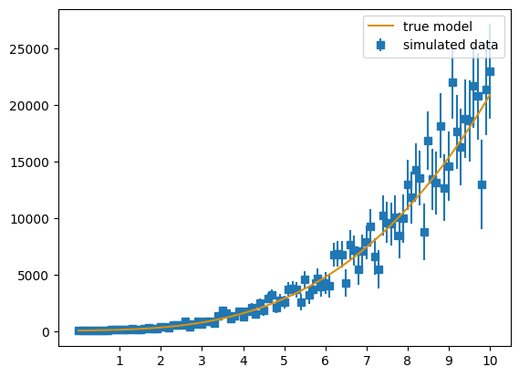
#Setting amount of data points
xmin = 0
xmax = 10
npoints = 101
xx = np.linspace(xmin, xmax, npoints)

#Choosing the model & simulating the data
model = true_model
yy, y_err = sim_data(xx)

#Setting maximum number of parameters
max_params = 10
params = np.arange(1, max_params+1, 1)
model = poly_model

#Plotting the simulated data and true model
plt.figure()
plt.errorbar(xx, yy, y_err, fmt='s', label='simulated data', zorder=1)
plt.plot(xx, true_model(xx), label="true model", zorder=2, color = '#de8f05')
plt.xticks(params)
plt.legend()
plt.style.use("seaborn-v0_8-colorblind")
plt.show()

#Calculating the likelihood and aic&bic the different amounts of parameters
aic = []
bic = []
for i in params:
    p0 = np.zeros(i)
    popt, pcov = curve_fit(model, xx, yy, p0=p0, sigma=y_err, absolute_sigma = False)
    pcov = np.sqrt(np.diag(pcov))
    log_L = log_gaussian_likelihood(model(xx, *popt), yy, y_err)
    aic.append(AIC(log_L, len(popt)))
    bic.append(BIC(log_L, len(popt), npoints))

#Plotting the results
plt.figure()
plt.subplot(1, 2, 1)
plt.plot(params, aic, marker="o", label="AIC")
plt.plot(params, bic, marker="o", label="BIC", color='#d55e00')
plt.xlabel("Number of parameters")
plt.xticks(params)
plt.title("AIC and BIC values")
plt.legend()
plt.subplot(1, 2, 2)
plt.plot(params[2:], aic[2:], marker="o", label="AIC")
plt.plot(params[2:], bic[2:], marker="o", label="BIC", color='#d55e00')
plt.xlabel("Number of parameters")
plt.xticks(params[2:])
plt.title("Zoomed in AIC and BIC values")
plt.legend()
plt.style.use("seaborn-v0_8-colorblind")
plt.show()
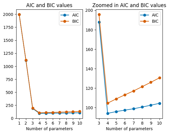
The resulting plot shows that the best fit model has 4 parameters, which of course is the right amount of parameters.
For the above simulation, we only calculated the likelihood once. In order to get the maximum likelihood, we will simulate the calculations multiple times, of which the maximum likelihood will be selected and used.
[23]:
#Simulate maximum likelihood estimation 101 times to find the maximum likelihood
N_sim = 101
aic = []
bic = []
for i in params:
    p0 = np.zeros(i)
    L = []
    for t in range(N_sim):
        model = true_model
        y, yerr = sim_data(xx)
        model = poly_model
        popt, pcov = curve_fit(model, xx, y, p0=p0, sigma=yerr, absolute_sigma = False)
        log_L = log_gaussian_likelihood(model(xx, *popt), y, yerr)
        L.append(log_L)
    #np.min is used to find the maximum likelihood. The logarithm is taken of the likelikhood, so the least negative log likelihood corresponds to
    #the highest likelihood.
    aic.append(AIC(np.min(L), len(popt)))
    bic.append(BIC(np.min(L), len(popt), npoints))

#Plotting the results
plt.figure()
plt.subplot(1, 2, 1)
plt.plot(params, aic, marker="o", label="AIC")
plt.plot(params, bic, marker="o", label="BIC", color='#d55e00')
plt.xlabel("Number of parameters")
plt.xticks(params)
plt.title("AIC and BIC values")
plt.legend()
plt.subplot(1, 2, 2)
plt.plot(params[2:], aic[2:], marker="o", label="AIC")
plt.plot(params[2:], bic[2:], marker="o", label="BIC", color='#d55e00')
plt.xlabel("Number of parameters")
plt.xticks(params[2:])
plt.title("Zoomed in AIC and BIC values")
plt.legend()
plt.style.use("seaborn-v0_8-colorblind")
plt.show()
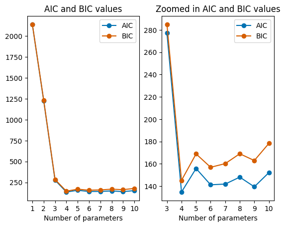
The above plot also shows the right amount of parameters. If you try running the code, there is a good chance that the lowest AIC and BIC values won’t be at 4 parameters, because of the likelihood function. Below the same calculation is done as for the plot above, but now multiple times to find the parameter which correspond to the lowest AIC and BIC values.
[31]:
#Simulating the calculations 101 times. In every simulation, the values are calculated 101 times.
#so if you run this code, it will take quite a long time

sim = 101
sim_range = np.arange(1, test+1, 1)
min_aic = []
min_bic = []

for n in sim_range:
    N_sim = 101
    aic = []
    bic = []
    for i in params:
        p0 = np.zeros(i)
        L = []
        for t in range(N_sim):
            model = true_model
            y, yerr = sim_data(xx)
            model = poly_model
            popt, pcov = curve_fit(model, xx, y, p0=p0, sigma=yerr, absolute_sigma = False)
            log_L = log_gaussian_likelihood(model(xx, *popt), y, yerr)
            L.append(log_L)
        aic.append(AIC(np.min(L), len(popt)))
        bic.append(BIC(np.min(L), len(popt), npoints))
    min_aic.append(np.argmin(aic)+1)
    min_bic.append(np.argmin(bic)+1)
[32]:
#Plotting the results
plt.figure()
plt.hist(min_aic, bins=params, align="left", alpha=0.5, label="AIC", edgecolor='#0173b2', hatch="///")
plt.hist(min_bic, bins=params, align="left", alpha=0.5, color="#d55e00", label="BIC", edgecolor="#d55e00")
plt.axvline(x=4, label="True value", color="black", linestyle="--")
plt.xlabel("Number of parameters")
plt.ylabel("Frequency")
plt.xticks(params)
plt.title("Outcomes multiple runs")
plt.legend()
plt.style.use("seaborn-v0_8-colorblind")
plt.show()
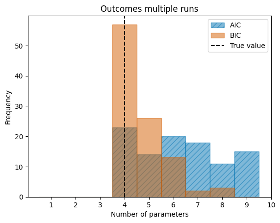
For this specific example, the BIC has a sharper peak in the frequency of finding the correct value than the AIC has. The plot also shows that both the AIC and BIC agree on 4 as the correct number of parameters most of the times.
Bootstrap and confidence intervals
The bootstrap method is a technique used to estimate a confidence interval (Chapter 1) for a parameter which inherently does not have a confidence interval. This is a powerful method since we do not need to know the distribution from which the data has been drawn.
Bootstrap method
Suppose you have a dataset with a large number of entries and you want to use Bayesian statistics to further develop a posterior likelihood. You need to have some distribution of your parameter which you can use later on, but you only have one dataset and thus one way to compute the parameter. The \(\textbf{bootstrap method}\) provides a way to develop a confidence interval for this parameter. It creates a new dataset from the original one with replacement, we do this by randomly selecting an entry from the dataset and putting it in our new dataset. In this way the new dataset is build up by a population of the original dataset. This specific bootstrap method is known as the \(\textbf{nonparametric bootstrap}\). The counterpart is the \(\textbf{parametric bootstrap}\), here we use the most likely parameter estimates from the original dataset to construct a new dataset. From there we find a most likely parameter and return this value. The parametric bootstrap fails if the original dataset is misspecified. However, the nonparametric bootstrap essentially always works!
The bootstrap algorithm works as follows:
Step 1: Simulate \(B \in \mathbb{N}\) independent datasets \(Y_{1,b}, ..., Y_{n,b}\) from the true distribution, for \(b = 1, ..., N\). Thus simulating \(B\) bootstrap samples.
Step 2: For each \(b\), compute the parameter \(\hat{\theta_b}\)
Step 3: Define your \(\gamma\)-confidence interval with the quantiles \(\hat{q}_{\alpha/2}\) and \(\hat{q}_{1-\alpha/2}\) for each parameter \(\hat{\theta_1}, ..., \hat{\theta_B}\)
Step 4: Define your confidence intervals
\[(\hat{\theta}_l, \hat{\theta}_u) = (\hat{q}_{\alpha/2}, \hat{q}_{1-\alpha/2})\]
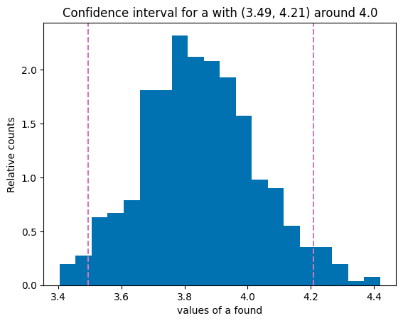
The next question we need to consider is the amount of bootstrap samples we need to use, thus how large does \(B\) need to be to get the quantile estimates \(\hat{q}_{\alpha/2},\hat{q}_{1-\alpha/2}\) to be stable. From multiple sources you can gather that finding a precise bootstrap sample size is not an exact science. Many say that 10.000 is a safe bet and thus this size. While many sources also mention that a sample size of 10.000 is also a very intense workload so for a quick test a sample size of 500 is all you need. So the question is how good you want your resolution to be, for a quick look into the confidence interval a sample of size of 500 is great and for an exact interval a sample size of 10.000 is recommend given your system can handle it.
[27]:
from scipy.optimize import curve_fit
import random

# Bootstrap exercise with sin(ax) as example
a_true = 4
b_true = 3

x_min = 0
x_max = 10
N = 100
x = np.linspace(x_min, x_max, N)

def linear(x, a=a_true, b=b_true):
    return a*x + b

model = linear
y_samp, y_unc = sim_data(x)

bootstrap_samples = 500

a_s = []
for i in range(bootstrap_samples):
    x_data = []
    y_data = []
    for i in range(N):
        temp = random.randint(0, (N-1))
        x_data.append(x[temp])
        y_data.append(y_samp[temp])
    popt, pcov = curve_fit(linear, x_data, y_data, absolute_sigma=True, maxfev=800)
    a_s.append(popt[0])

# In our variable a_s we have a distribution of a's found by the bootstrap model.
# Now we need to determine our gamma-confidence

gamma = 95

z = z_alpha(gamma)

mean_a = np.mean(a_s)
std_a = np.std(a_s)

lower = mean_a - z*std_a
higher = mean_a + z*std_a
# Now that we have the confidence interval, all we need to do is plot it

plt.hist(a_s, bins = 20, density=True)
plt.axvline(lower, color='#cc78bc', linestyle="--", label=f"Lower limit {gamma}%")
plt.axvline(higher, color='#cc78bc', linestyle="--", label=f"Upper limit {gamma}%")
plt.title(f"Confidence interval for a with ({lower.round(2)}, {higher.round(2)}) around {np.round(mean_a)}")
plt.ylabel("Relative counts")
plt.xlabel("values of a found")
plt.style.use("seaborn-v0_8-colorblind")
plt.show()