Chapter 1: Hypothesis Testing & Maximum Likelihood

Hypothesis Testing

A hypothesis is a statement regarding a population parameter. The hypothesis test is used to make a decision, based on a sample from the population, which of the hypotheses is true; either the Null hypothesis or the Alternative hypothesis.

The null hypothesis is the default assumption that there is no relationship between two measured phenomena and is denoted as \(H_0\). The alternative hypothesis is the complement of the null hypothesis and is denoted as \(H_1\). Let us note this in a more formal mathematical manner.

Let \(\theta\) denote the hypothesis and let us partition the parameter space \(\Theta\) into two complementary sets, \(\Theta_0\) and \(\Theta_1\), such that \(\Theta_0\)+\(\Theta_1\)=\(\Theta\). The hypothesis test tests

\[H_0:\ \theta\in\Theta_0\ \text{versus}\ H_1:\ \theta\in\Theta_1.\]

For example, \(\theta\) may characterize the shift in frequency of light due to differences in velocities of an observer and source (Doppler shift). A sceptical astronomer may be interested to see whether the Doppler shift exists or not. The null hypothesis may then be \(H_0: \theta = 0\), implying that there is no shift in frequency while the alternative hypothesis may be \(H_1: \theta \neq 0\).

Sticking with this example, if the sceptical astronomer researches this hypothesis thoroughly (with perfect equipment), they will of course find that \(\theta\neq0\) since the Doppler effect exists. Hence, the astronomer should reject the Null hypothesis. Suppose the sceptical astronomer uses faulty equipment and finds \(\theta=0\), they should then (wrongfully) retain the Null hypothesis.

This wrongful retention is one of the two errors that can be made in hypothesis testing. Them being a type I error and type II error. A type I error occurs when the Null hypothesis is rejected when in reality it is true. A type II error occurs when a Null hypothesis is accepted while in reality it is false. In the latter example the astronomer thus makes a type II error, since the Doppler effect is real and thus there is a shift in frequency implying that the Null hypothesis should be rejected. These errors have been summarized in the table below.

	Retain Null	Reject Null
H₀ true	Correct	Type I error
H₁ true	Type II error	Correct

It should be noted that a null hypothesis can never be accepted. For that to happen, an infinite number of measurements must be made, which is of course impossible. It is only possible to find evidence against the null hypothesis.

To test a hypothesis a Test Statistic (TS) should be made. The test statistic is then used to measure the probability of a measurement outcome, given that the null hypothesis is true. This probability is also known as the p-value discussed in the next subsection.

The test statistic can be any statistic that combines multiple random variables into a single number. This can be for example the median of a dataset, a likelihood ratio, etc. If the probability distribution of the test statistic is known from theory, a probability can be assigned to a given test statistic. If the probability distribution is unknown, Monte Carlo simulations can be used assuming \(H_0\) is correct. More on this in chapter 6.

p-values

As briefly introduced in the previous subsection, the p-value can be defined as follows:

\[\boxed{\textit{the p-value is the probability of measuring a dataset $Y$ if the null hypothesis is correct.}}\]

The p-value is derived from the test statistic which is some function that maps the dataset \(Y\) to a single value. More precisely, it is derived from the probability distribution of the test statistic known from theory or from a Monte Carlo simulation.

The null hypothesis is rejected if the test statistic falls within a predetermined region, called the rejection region. Often in literature this rejection region is set at a value for the test statistic, such that the corresponding p-value is less than \(0.05\). This limiting value is often called the significance.

In scientific articles, often something along the lines of “this null hypothesis is rejected at the \(n\ \sigma\) level” is stated. This simply means that the observed result is significant to a degree where the probability of it occurring due to random chance corresponds to a deviation of \(n\sigma\) from the mean of a normal distribution. For example: \(1\ \sigma\) would correspond to a confidence level of \(68.3\%\), \(3\ \sigma\) corresponds to \(99.7\%\), etc.

Advantages and Disadvantages of Hypothesis Testing

The main advantage of hypothesis testing is that it provides a structured framework for decision-making. The steps of hypothesis testing are as follows:

1. Form a null and alternative hypothesis.

2. Define a test statistic \(T\).

3. Find the probability distribution of the test statistic.

4. Compare the test statistic with the probability distribution to find the p-value.

In addition, the concept of p-values is widely known across disciplines.

Hypothesis testing has some notable downsides. One major issue is that statistical tests are often applied more than necessary. In many situations, confidence intervals or estimation methods might be more appropriate. If you don’t have a clear, meaningful hypothesis, don’t need to make a definitive yes-or-no decision, or aren’t concerned about error probabilities, then hypothesis testing might not be the right approach for your needs.

Another issue around p-values is the misinterpretation of them. The p-value is not the probability of \(H_0\) being correct. This is a mistake often found in articles. It is strictly the probability of measuring a dataset \(Y\) if the null hypothesis is correct based on the defined test statistic (with explicit emphasis on the word if). The true definition of the p-value is thus a bit of an awkward one and should therefore be used with caution when communicating with a wider audience consisting of not only those educated in statistics.

Scientific fields like psychology and medicine have faced a major challenge called the replication crisis due to this misinterpretation of p-values. Here, many high-profile findings couldn’t be reproduced, even with large samples and identical methods. This revealed that a significant number of “discoveries” might actually be false positives, despite being widely accepted and forming the basis of extensive research. Several factors contribute to this problem, both unintentional and deliberate:

1. Multiple Testing: Many studies fail to account for the fact that testing multiple hypotheses increases the likelihood of false positives. This oversight is often due to inadequate education in statistics.

2. Publication Bias: Journals prioritize significant results, leading to the “file drawer effect”, where studies with non-significant findings remain unpublished. As a result, the scientific record is biased toward positive results.

3. Incentives and Misconduct: Researchers may unintentionally or deliberately engage in practices like:

   • HARKing (Hypothesizing After Results are Known): Creating hypotheses based on the data after seeing the results, which undermines the validity of the conclusions.

   • p-hacking: Manipulating data or analysis (e.g., excluding outliers or changing variables) to achieve statistically significant results.

These issues have started to gain attention in recent years, prompting efforts to improve research practices. While fields like astronomy and physics have been less affected, they are not immune. The lesson is clear: small shortcuts or biases can accumulate and harm the integrity of science.

Example: sceptical astronomer

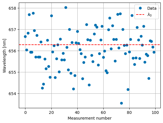
Let’s return to the example of the sceptical astronomer. Suppose the astronomer has a dataset of \(N=100\) measurements of the Doppler shift. He lets the velocity difference between the observer and source be \(50 \text{ km s}^{-1}\). Let us assume that the source is a hydrogen atom transitioning from the \(n=3\) to the \(n=2\) orbital, generating a photon with a wavelength of \(\lambda_0=656.279\text{ nm}\). The astronomer wants to test the hypothesis that the Doppler shift is zero. Since this is an illustration of hypothesis testing, we will generate the data using the Doppler shift formula and then perform a hypothesis test on it.

Let us assume the uncertainty in the measurements is due to the equipment and is \(1\text{ nm}\) (a relatively large uncertainty when the shift will be around \(0.1\text{ nm}\)). We will generate the data and plot it below.

import numpy as np
import astropy.constants as c
import astropy.units as u
import matplotlib.pyplot as plt

# LaTeX rendering
plt.style.use("seaborn-v0_8-colorblind")

def doppler_shift(dv, f_0):
    return (1+dv/c.c)*f_0

# Generate some data
np.random.seed(42)

# Balmer alpha line
lambda_0 = 656.279*u.nm

# Doppler shift
f_0 = c.c/lambda_0
dv = 50*u.km/u.s
f = doppler_shift(dv, f_0)

# Convert to wavelength
lam = c.c/f

# Add noise
noise = np.random.normal(0, 1, 100) * u.nm
data = lam + noise

plt.plot(data, 'o', label='Data')
plt.xlabel('Measurement number')
plt.ylabel('Wavelength [nm]')
plt.grid()
plt.axhline(lambda_0.value, color='r', linestyle='--', label=r'$\lambda_0$')
plt.legend()
plt.show()

We can use the test statistic \(T\) as the mean of the data. The p-value is then the probability of measuring a dataset with a mean equal to or more extreme than the observed mean, given that the null hypothesis is true. We will perform this test below.

A test statistic \(T\) of this form can be defined as

\[T = \frac{\text{Observed statistic}-\text{Expected statistic}}{\text{Standard deviation of statistic}} \tag{1.1}\]

In this case, the expected statistic is the mean of the data under the null hypothesis (\(\lambda_0\)), the observed statistic is the mean of the data, and the standard deviation of the statistic is the standard deviation of the data divided by the square root of the number of measurements.

from scipy.stats import norm

# Compute the standard error (SE) assuming constant measurement uncertainty
std_dev = np.std(data)          # Standard deviation of our simulated data
n = len(data)                   # Number of observations
se = std_dev / np.sqrt(n)       # Standard error

# Compute the observed test statistic
T = (np.mean(data) - lambda_0) / se

# Calculate the two-tailed p-value
p_value = 2 * (1 - norm.cdf(abs(T)))

print(f'Test statistic: {T:.2f}')
print(f'p-value: {p_value:.5e}')

Test statistic: -2.36
p-value: 1.82584e-02

Let’s recap for a minute what we have done. We have generated a dataset of 100 measurements of the Doppler shift of a hydrogen atom. We have then calculated the test statistic \(T\) as the mean of the data and the p-value as the probability of measuring a dataset with a mean equal to or more extreme than the observed mean, given that the null hypothesis is true. We found that the p-value is \(1.8\%\). This is a small probability given that our uncertainty per measurement is \(1\text{ nm}\) and only 100 datapoints were simulated.

Maximum likelihood

Before we can talk about the maximum likelihood estimation, we need to take at look at parametric models and parametric inference. A parametric model has the form

\[\mathcal{F} = \{f(y;\theta) : \theta \in \Theta\}\]

where \(\Theta \subset \mathbb{R}^k\) is the parameter space and \(\theta = (\theta_1,..., \theta_k)\) is the parameter, meaning \(\Theta\) is a \(k\)-dimensional parameter space with real numbers for each parameter and \(\theta\) is a specific point in this parameter space. The goal of inference is now to estimate the specific value of \(\theta\) that best represents the true parameter \(\theta^*\) based on the observed data \(Y_1,...,Y_k\). This specific value of \(\theta\) will be called \(\hat{\theta}\). To find this \(\hat{\theta}\), it is natural to ask:

\[\textit{Given observed data $Y_1, . . . , Y_n$, which value for the true parameter $\theta^*$ is most probable?}\]

However, the problem here is that \(\theta^*\) is a fixed unknown value, while we want to assess it to a probability. This is unfortunately not possible in the frequentist framework. To fix this, we need to use a Bayesian framework and we must ask a different question.

\[\textit{Given a parameter value $\theta$, how probable is it that we observe the data $Y_1, . . . , Y_n$?}\]

Now the data can be assets probabilistically, as they are random variables. The estimator \(\hat{\theta}\) is then defined as the value of \(\theta\) at which the data is the most likely; so given the parameter, we maximize the likelihood.

This maximum likelihood estimation is the most common method for parameter estimation in a parametric model. Before moving forward, we first need to define the likelihood of the data.

If we compute Independent and Identically Distributed (IID) values \(Y_1,...,Y_n\) with a PDF \(f(y;\theta)\), the likelihood function is defined by:

\[\mathcal{L}_n(\theta) =\prod_{i=1}^{n} f(Y_i;\theta) \tag{1.2}\]

Therefore, the log-likelihood function is then defined by: \(\ell_{n}(\theta)=\log\mathcal{L}_n(\theta)\)

Maximum Likelihood Estimator

The maximum likelihood estimator (MLE) :math:`hattheta` is defined by the value of \(\theta\) that maximizes \(\mathcal{L}_n(\theta)\). This value of \(\hat\theta\) is the same for both \(\mathcal{L}_n(\theta)\) and \(\ell_{n}(\theta)\), as the maximum of a function occurs at the same place as the maximum of the logarithm of this function. This is especially convenient if we look at the maximum likelihood estimator in a mathematical way. The MLE of the likelihood is defined with a product.

\[\hat{\theta} = \arg \max_{\theta \in \Theta} \prod_{i=1}^{n} f_{\theta}(Y_i). \tag{1.3}\]

So the MLE of the log-likelihood is then defined with a sum.

\[\hat{\theta} = \arg\max_{\theta \in \Theta} \sum_{i=1}^{n} \ln f_{\theta}(Y_i) \tag{1.4}\]

Once you recall that the maximum of a function is found by setting the first derivative of a function equal to zero, the advantage of the log-likelihood function is easily seen. Indeed, the derivative of a sum is the same as the sum of the derivatives. While the derivative of a product of n terms will result in applying the product rule n times.

The MLE can be computed theoretically. This is done by the following steps:

1. Computing the log-likehood function \(\ell_{n}(\theta)\)

2. Calculate the first derivative of each component

3. Set all the derivatives to zero. For an \(n\)-dimension \(\ell_{n}(\theta)\) this gives

   \[\frac{\partial \ell(\theta)}{\partial \theta_1} = 0 \quad , ..., \quad \frac{\partial \ell(\theta)}{\partial \theta_n} = 0. \tag{1.5}\]

4. Solve the equations from step 3 so that MLE \(\hat{\theta}\) of \(\theta\) is found.

Sometimes, these steps can be a lot of computation work. If you don’t feel like doing this or a statistical problem is simply too difficult, you can also determine the MLE numerically. In a Python script, this can for example be done with the scipy.optimize module. The following example demonstrates that there is no disparity between computing the MLE analytically or numerically.

Example: Analystical versus Numerarical MLE

Consider the probability density function

\[f(\mu, \sigma) = \frac{1}{\sqrt{2\pi} \sigma} e^{-\frac{(y - \mu)^2}{2\sigma^2}}. \tag{1.6}\]

This gives the log-likelihood function

\[\ell(\mu, \sigma) =\sum_{i=1}^{N} \ln(f(\mu,\sigma)) =-\frac{N}{2} \ln(2\pi) - N \ln(\sigma) - \frac{1}{2\sigma^2} \sum_{i=1}^{N} (y_i - \mu)^2. \tag{1.7}\]

For this log-likelihood function \(\ell(\mu, \sigma)\) the maximum likelihood is calculated both analytically and numerically. Let’s assume the data from the example above regarding the sceptical astronomer (notice how the data variable is not changed in this piece of code and is used directly from the previous example). Run the Python script below to see that the same value of the MLE is found regardless of which computation is used.

import numpy as np
from scipy.optimize import minimize
# Define random data points and the number of data points
N = len(data)

# We define a function to calculate the MLE analytically
def analytical(data):
    # mu_hat is defined by the mean of the data, because f is defined as a normal distribution.
    mu_hat = np.mean(data)
    # Define sigma_hat
    sigma_hat = np.sqrt(np.mean((data - mu_hat) ** 2))

    return mu_hat, sigma_hat


# We define a function to calculate the MLE numerically
def numerical(data):
    # Define the negative log-likelihood function, so that we can use scipy.optimize.minimize
    def negative_log_likeli(parameters):
        mu, sigma = parameters
        # Ensure that sigma is not negative
        if sigma <= 0:
            return np.inf
        # Return the negative log-likelihood function
        return N / 2 * np.log(2 * np.pi) + N * np.log(sigma) + np.sum((data - mu) ** 2) / (2 * sigma ** 2)

    # Convert the data to dimensionless values so scipy can work with it
    data = data.value
    # Take a first guess for the numerical solution
    mu_guess = 0
    sigma_guess = 1

    # Minimize the negative log-likelihood function to get mu and sigma
    parameters =  minimize(negative_log_likeli, [mu_guess,sigma_guess], method="L-BFGS-B", bounds=[(-np.inf, np.inf), (1e-6, np.inf)])

    # We don't convert units in the minimization process, hence the units that the values originally had return
    mu_numerical = parameters.x[0] * u.nm
    sigma_numerical = parameters.x[1] * u.nm

    return mu_numerical, sigma_numerical

mu_analytical, sigma_analytical = analytical(data)
mu_numerical, sigma_numerical = numerical(data)

print("Analytical method:")
print(f"\u03BC = {mu_analytical}, \u03C3 = {sigma_analytical} \n")

print("Numerical method:")
print(f"\u03BC = {mu_numerical}, \u03C3 = {sigma_numerical}")

Analytical method:
μ = 656.0657161793672 nm, σ = 0.9036161766446291 nm

Numerical method:
μ = 656.0657163204406 nm, σ = 0.9036161879095135 nm

The question you may now have as to why the MLE is such a commonly used estimator. The case is that the MLE has several nice quantities like consistency, which we will not dive into here. However, one reason we can name to use the MLE, is that no other estimator has a smaller variance and thus the MLE extracts the maximum information. In a simpler way one of the most famous statisticians said:

\[\textit{''It's just common sense.'' — Pierre-Simon Laplace.}\]

On the other hand, we should always beware when to use which statistical model and if this model is correctly specified. If some of your parameters are poorly identified, the estimate model will not converge to the actual one. In this case, it is so much that the statistical model is wrong, but rather that it is not useful. An example is the stock market crash in 2008, where the losses of the Dow Jones Industrial Average were more than seven \(\sigma\). This indicates that the losses were more than seven times higher than the standard deviation. The probability of this happening is around \(2 \cdot 10^{-8}\). It is not that we are very unlucky that this happened despite this small chance, but there are more parameters at play, which are not incorporated in our model. Therefore, our model was not applicable this time.

Least squares

The least square method is a parameter estimation method based on minimizing the sum of the squares of the residuals. This method is closely related to the MLE method. Especially if our parametric model has the form of a normally distributed PDF, like in the example above. Here the MLE was found by maximizing the same log-likelihood function as Eq 1.8:

\[\ell(\theta) =-\frac{N}{2} \ln(2\pi) - N \ln(\sigma) - \frac{1}{2} \sum_{i=1}^{N} \frac{(y_i - f(x_i,\theta))^2}{\sigma_i^2}. \tag{1.8}\]

This is equivalent to minimizing the negative of this log-likelihood function. Ignoring the constants that do not depend on \(\theta\), you end up with Eq 1.9. This formula is the statistic, the sum of the squares of the residuals, that we need to minimize for the least square method with an additional weight factor.

\[\chi^2 = \sum_{i=1}^{N} \frac{(y_i - f(x_i,\theta))^2}{\sigma_i^2} \tag{1.9}\]

Due to the extra weight factor, the minimisation of this statistic would be called the weighted least square method. When the weight factor is equal to \(\frac{1}{\sigma^2}\) the weighted least square method is also referred to as the chi-square (:math:`mathbf{chi^2}`) minimization. When \(\sigma\) is unknown or \(\sigma\) is the same for each data point, Eq 1.10 is used as the statistic to be minimized of the ‘normal’ least square method.

\[\chi^2 = \sum_{i=1}^{N} (y_i - f(x_i,\theta))^2 \tag{1.10}\]

There are some problems with the least square and thus chi-square method. As we have seen these two methods are the same as the MLE if the PDF is normally distributed. Therefore, it is assumed that the error follows a normal distribution. A problem now arises, if the data errors are not Gaussian, the least squares method is no longer optimal. On the other hand, the MLE allows you to specify and alter the likelihood function based on the correct error distribution.

Another problem with the least square method is that it does not allow you to compare different models. While alternatively the MLE is often used with tools like the Akaike Information Criterion (AIC) or Bayesian Information Criterion (BIC) for model comparison. More on these tools will be discussed in Chapter 2. Despite these problems the least square and chi-square method are widely used and therefore it is important to know them, but whenever you can, use the Maximum Likelihood Estimation.

Generative model

When fitting a model to data the same question always arises: “Is my fitting procedure justifiable?” The answer is often debatable. Luckily there is a consistent and scientifically justifiable way to do this, a generative model. A generative model is parametric, quantitive description of a statistical process that could have generated the observed data. Let’s start with an example (from Hoggs et al. 2010).

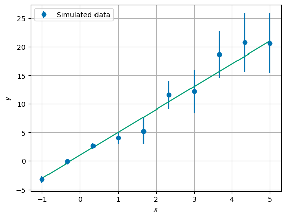
Imagine you have a dataset \(Y\) of \(N\) data points, which you want to be able to explain using a model. We expect that the data comes from a linear model,

\[f(x)=ax+b.\]

We have observed the dataset {\(y_i\)} with uncertainties {\(\sigma_{y_i}\)}. Our goal is to find the parameters that are most likely to have generated our data, given this model. We can do this by writing down a generative model. This model should be a description of a statistical procedure that could have realistically generated the known dataset. For this example, we say that the {\(y_i\)} are drawn from a Gaussian distribution with uncertainties {\(\sigma_{y_i}\)} and a mean following a straight line. So the data deviates from a straight line with small offsets drawn from a Gaussian distribution. Now we can create a distribution which describes the probability that the points \(y_i\) lie on the described interval, given the knowledge that we have:

\[p(y_i|x_i,\sigma_i,a,b)=\frac{1}{\sqrt{2\pi\sigma_i^2}}e^{-\frac{(y_i-ax_i-b)^2}{2\sigma_i^2}}, \tag{1.11}\]

where {\(x_i\)} are the independent positions, \(a\) is the slope, \(b\) is the intercept and \(y_i\) and \(\sigma_{y_i}\) are defined as before. Now that we have this distribution, we can achieve our goal of finding the parameters that are most likely to have generated our data. The total probability of finding of the complete set \(Y\) given our prior knowledge and the fact that the points are IID, is simply given by the likelihood (Eq. 1.2):

\[\mathcal{L}=\prod_{i=1}^Np(y_i|x_i,\sigma_i,a,b). \tag{1.12}\]

Now, using Bayes’ Theorem, we can write down:

\[p(a,b | \{y_i\}^N_{i=1}, I) \propto p(\{y_i\}^N_{i=1}|a, b, I)p(a,b|I) \tag{1.12},\]

where \(I\) is a shorthand for all the knowledge we have beforehand, \(p(a,b | \{y_i\}^N_{i=1}, I)\) is the posterior distribution, \(p(\{y_i\}^N_{i=1}|a, b, I)\) is the likelihood from before and \(p(a,b|I)\) is the prior distribution for the parameters.

Let’s work out this example using Python.

# We start by generating data
import numpy as np
import matplotlib.pyplot as plt
plt.style.use('seaborn-v0_8-colorblind')
a_true = 4
b_true = 1
x = np.linspace (-1, 5, 10)

def line_model(x, a, b):
    return a*x + b

def generate_data(x):
    y_true = line_model(x, a_true, b_true) #The true y values according to the model
    y_uncert = np.abs(y_true * np.random.uniform(0.2, 0.3, len(x))) #Generate fractional uncertainties with fractions between 0.2 and 0.3
    y_gen = np.random.normal(y_true, y_uncert) # Generate artificial data
    return y_gen, y_uncert

def likelihood(a, b, x, y_gen, y_uncert): #Defining the likelihood
    return (np.prod(1/(np.sqrt(2*np.pi*y_uncert**2))*np.exp(-((y_gen -a*x -b)**2)/(2*y_uncert**2))))

y_gen, y_uncert = generate_data(x)

plt.errorbar(x, y_gen, yerr=y_uncert, fmt='o', label='Simulated data')
plt.plot(x, line_model(x, a_true, b_true))
plt.xlabel(r'$x$')
plt.ylabel(r'$y$')
plt.grid()
plt.legend(loc='upper left')
plt.show()

Now, let us find the probability of different values of \(a\) and \(b\). Here we define the prior distribution \(p(a,b|I)\) as uniform for each combination of \(a\) and \(b\), as long as \(2 \leq a \leq 6\) and \(-1 \leq b \leq 3\).

dist = []
parameters = []

for a in np.arange(2, 6, 0.1):
    for b in np.arange(-1, 3, 0.1):
        dist.append(likelihood(a, b, x, y_gen, y_uncert)) # Calculate the likelihood for each combination of a and b
        parameters.append([a,b])

parameters = np.asarray(parameters)

plt.scatter(parameters[:,0], parameters[:,1], c=dist, cmap='binary' )
plt.xlabel(r'$a$')
plt.ylabel(r'$b$')
plt.axvline(a_true, c='r')
plt.axhline(b_true, c='r')
plt.title('Probabilities of Each Parameter Combination')
plt.colorbar(ticks=[], label='probability')
plt.grid()

a_found = parameters[np.where(dist == np.max(dist)),0][0][0]
b_found = parameters[np.where(dist == np.max(dist)), 1][0][0]

print(f'We find the most likely parameters to be: a={a_found:.1f}, b={b_found:.1f}')

We find the most likely parameters to be: a=4.0, b=1.2

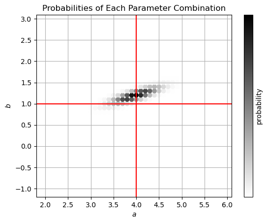
In the figure we can see that the probability distribution gives a good estimation for \(a\) and \(b\). We have seen that the generative model gives a good foundation for the posterior distribution. In practice, it often comes down to maximizing the likelihood or minimizing the \(\chi ^2\)-value. Using a generative model allows for reproducable results and is scientifically justifiable. Additionally, this method is applicable in many different cases. However, the complexity of models quickly increases in the case of, for example, non-linear relations. The generative model requires assumptions about the data and the uncertainties. Luckily, in practice these assumptions are usually justifiable and derivable from the measurement procedure.

Confidence intervals

One of the most popular ways to communicate uncertainty is through confidence intervals. The idea is to find an interval around the estimated value \(\hat\theta\) that covers the true value \(\theta^*\). We characterize the confidence interval through the confidence level :math:`gamma`. A \(\gamma\)-confidence interval has a probability of at least \(\gamma\) that the interval \((\hat\theta_l,\hat\theta_u)\) contains the true parameter \(\theta^*\), or in mathematical terms:

\[P(\theta^*\in(\hat\theta_l,\hat\theta_u)\geq\gamma \tag{1.13}\]

It is important to realize that you do not say you are, for example, \(95\%\) sure that the found \(\hat\theta\) is the true value, but you say that you are \(95\%\) sure the true value lies on the interval \((\hat\theta_l,\hat\theta_u)\).

The most straightforward way to compute the confidence interval is using the following procedure, where \(se\) is the standard error:

If \(\hat{\theta} \approx N({\theta}^{*}, se[\hat{\theta}]^2)\) and \(\hat{se}[\hat{\theta}] \rightarrow_p se[\hat{\theta}]\), the interval

\[(\hat{\theta}_l, \hat{\theta}_u) = (\hat{\theta} - z_{\alpha/2} \hat{se}[\hat{\theta}], \hat{\theta} + z_{\alpha/2} \hat{se}[\hat{\theta}]) \tag{1.15}\]

is an approximate \((1-\alpha)\)-confidence interval where \(z_{\alpha/2}\) are the corresponding quantile coming from \(\gamma = 1 - \alpha\).

Below an example using a normal distribution is given.

import numpy as np
from scipy.stats import norm
import matplotlib.pyplot as plt

# Here we generate some data like a normal distribution
mu, sigma = 2, 1
x = np.random.normal(mu, sigma, 1000)
x.sort()

gamma = 90 #The confidence we choose
gamma2 = 95

# Calculate the z value
def z_alpha (gam):
    alpha = 1-(gam/100)
    z = norm.ppf(1-(alpha/2))
    return z

z = z_alpha(gamma)
z2 = z_alpha(gamma2)

lower1 = mu - z*sigma
upper1 = mu + z*sigma

lower2 = mu - z2*sigma
upper2 = mu + z2*sigma


print(f"The actual confidence interval would be ({lower1.round(2)}, {upper1.round(2)}) for a gamma of {gamma}%")
print(f"The actual confidence interval would be ({lower2.round(2)}, {upper2.round(2)}) for a gamma of {gamma2}%")

plt.title("Example of a confidence interval using normal distribution")
plt.hist(x, 30, density=True, color="royalblue")
plt.plot(x, 1/(sigma * np.sqrt(2 * np.pi)) * np.exp( -1 * (x - mu)**2 / (2 * sigma**2) ),linewidth=2, color='darkorange')
plt.axvline(lower1, color = 'limegreen', linestyle="--", label=f"Lower limit {gamma}%")
plt.axvline(upper1, color = 'limegreen', linestyle="--", label=f"Upper limit {gamma}%")
plt.axvline(lower2, color="violet", linestyle="--", label=f"Lower limit {gamma2}%")
plt.axvline(upper2, color="violet", linestyle="--", label=f"Upper limit {gamma2}%")
plt.legend()
plt.grid()
plt.show()

The actual confidence interval would be (0.36, 3.64) for a gamma of 90%
The actual confidence interval would be (0.04, 3.96) for a gamma of 95%

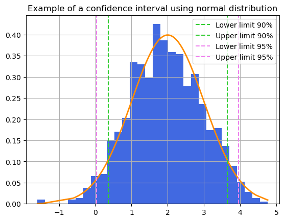
As you can see from the example, the larger \(\gamma\) the larger the area in which you can find your parameter.

Sources:

• Hogg, D., Bovy, J., Lang, D., 2010, Instrumentation and Methods for Astrophysics,arXiv preprint arXiv:1008.4686.

• Casella, G., Berger R., 2002, Statistical Inference, Second edition

• Wackerly, D., Mendenhall, W., Scheaffer, R., 2008, Mathematical Statistics with Applications, Seventh Edition

• Wasserman, L., 2004 All of Statistics, First Edition

• Disorbo, M., 2017, Inference!

• Hogg, R., Tanis, E., Zimmerman, D., 2013, Probability and Statistical Inference, Ninth Edition

• Taylor, J., 1982, An Introduction to Error Analysis, Second edition